I recently decided to convert my AHRS algorithm in the STorM32 gimbal controller firmware from floating-point to fixed-point arithmetic. It requires the trigonometric functions  ,
,  ,
,  , and
, and  , as well as the square-root
  or inverse square-root
  . Thus, I scanned the web for fast implementations, and google of course produced many hits. However, none of the pages and/or libraries provided solutions which satisfied my needs. So, I developed my own algorithms, which I like to share below.
1. Fast Sin and Cos
2. Fast Atan2
3. Fast Arcsin
4. Fast Inverse Sqrt
Before diving into the details, I’d like to first add some comments on „my needs“.
1) The target microcontroller is a STM32 F1, with 32-bit Cortex-M3 core. At this point you may ask: Why not going ahead and using a STM32 F3 or STM32 F4, which offer a FPU? Well, true, their FPU is amazing. However, it doesn’t provide trigonometric functions, and the compiler built-in functions won’t be very fast either. Also, I find the F4 quite expensive (I would run mad then I would destroy F4’s in my tinker work). So, I’m with the F1. However, F3/F4 users should also profit from the algorithms below, since they can also be directly applied to float and would be faster than the float built-in functions.
2) The above functions can all be done with CORDIC. However, besides being renowned for being slow, a major obstacle is IMHO its irregular error behavior. This leads to substantial noise in e.g. calculated derivatives, needed in PID controllers. It was hence clear to me from the outset that only polynomial approaches (such as polynomial approximation, Chebyshev approximation, minimal polynom, rational approximation, Pade series, Taylor or Laurent series expansion) come into question, since their error function is smooth. Then the relative precision is much higher than the absolute accuracy. In addition, the STM32 core provides single-cycle multiplication, and calculating polynomials is very fast. For this reason also look-up tables were not considered, since in the time two data points are loaded from memory many multiplications may be done.
3) I aimed at an absolute precision better than 0.01°, or  with respect to 360°, which is about 16 bit resolution. Otherwise the gimbal controller wouldn’t work as accurate as I want it to. This requirement alone ruled out essentially all approximations found on the web, since none did come close to this.
4) The application target of AHRS calculations sets further demands. For instance, one nearly always needs both the sine and cosine of an angle. Hence, the combined time for calculating both is relevant for evaluating an algorithm. Similarly,  should show a proper error behavior, and e.g. not exceed 1.
5) On the other hand, AHRS calculations lend themselves perfectly to fixed-point arithmetic, since all values are bounded by one. Floating-point is in fact a waste here, and with the proper fixed-point format even better numerical accuracy is obtained. The widely used Q16 fixed-point format is however ruled out by the required 16 bit absolute precision – in order to cope with numerical errors one should have some extra bits of precision in the calculations. The floating-point code with its 23-bit mantissa works very well, which suggests the Q24 format. However, most AHRS calculations involve numbers in the  range, and the Q31 format seems ideal. It’s much smarter though to allow for a
  range, since values might be momentarily somewhat larger than 1, which can easily be handled this way. Hence, I opted for the Q30 fixed-point format, and Q24 in the few cases where it is needed.
We are thus looking for fast codes, which provide an absolute accuracy of about  , are based on polynomials, and can be represented in a Q30 format. The algorithms below serve my purpose. However, for other applications they may not be „optimal“ (in whatever sense).
A final comment: Usually I take great care in referencing properly the sources from which I took relevant ideas. This time I however won’t. I went through so many pages and documents that I just can’t remember anymore where I found which idea. You may google them yourself.
1. Fast Sin and Cos
There are quite some interesting pages on the web on how to approximate e.g. the sine by polynomials (e.g. here, here, here, here, here). However, often the sine is approximated, and the cosine calculated from relations such as

(or vice versa). That’s not good, one might get both the sine and cosine with little additional cost. One frequently cited idea is to use a fast code for  and these relations
 ,
,  ,
, 
This looks smart, since one seemingly has to do only one costly calculation. However, two divisions are involved, and although the STM32 provides a hardware divider, a division may require up to 12 cycles (i.e. 12 multiplication and/or addition could be done). The most appealing idea I’ve seen is to exploit the mirror symmetry of and around  in the first quadrant (argument values
  ). The rational is that the polynomial approximation for the cosine can then be obtained from the sine approximation by simply reversing the signs of the odd terms. Both the sine and cosine are thus obtained for free, i.e. by simple subtraction and addition of the even and odd parts of the polynomial.
In detail: The angle range  is normalized to the range
  via the transformation

|
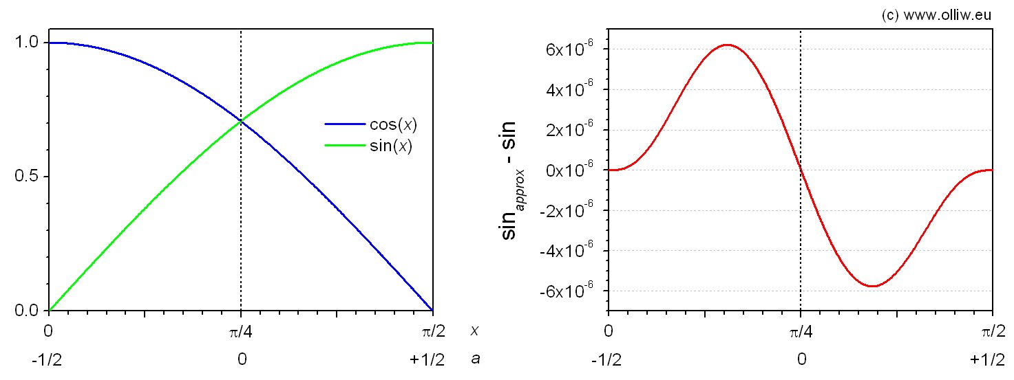
The polynomial approximations for the sine and cosine in the variable  read then


In practice one first calculates the even and odd parts,
 
|
from which both the sine and cosine values are trivially obtained:
 
|
A polynom of 6th order was required in order to achieve the accuracy requirement. Several minimization schemes for finding the coefficients where exploited (such as minimax, Chebyshev, and others), but they all produced results I didn’t like (mainly because the error wasn’t zero and/or smooth at the „edges“  , which relate to the 0° and 90° points). I thus determined the coefficients by requiring that the values, slopes and curvatures at match the real functions, as well as the value at
  . This yields the coefficients
   
|
  
|
The absolute error is smaller than  , and never exceeds 1. Only 7 multiplications and 7 additions are required.
It should also be noted that the coefficients are in the Q30 range and have alternating sign, such that overflow doesn’t occur in the evaluation of the polynomial (using of course Horner’s scheme).
The algorithm needs a wrapper, which identifies the quadrant of the angle  and maps it into the
  range. This may be achieved in various way (I might not have found the „best“ code), and it also depends on the format in which the angle is supplied. I represent the angle normalized to
  in Q24 format, such that 360° corresponds to +1. The code then reads (the 2nd and 3rd lines could be optimized further):
   //the quadrant is contained in the integer part plus two bits

   quadrant = (angle>>22) & 3;

   //the remainder is contained in the fractional part minus two bits

   angle = (angle<<2) & 0x00FFFFFF;

   //make it q30 fixed point and shift to range -1/2 ... 1/2

   a = (angle<<6) - Q30(0.5);

   // calculate sin&cos

   q30_sincos_normalized( a, &s, &c );

   // correct for quadrant

   switch( quadrant ){

     case 0: sin =  s; cos =  c; break;

     case 1: sin =  c; cos = -s; break;

     case 2: sin = -s; cos = -c; break;

     case 3: sin = -c; cos =  s; break;

   }
2. Fast Atan2
As for the sine and cosine the web retrieved many interesting pages also for the arctan (e.g. here, here, here, here). The algorithms generally reduce the problem to calculating the arctan in the range  . The values for
  are then obtained using formulas such as
 ,
, 
where the first is IMHO to be preferred since it avoids the sqrt. An alternative is to branch into  and
and  , and map the
  argument range onto using the transformation

and the inverse of it for (to ensure  ). This transformation may seem odd, but is in fact suggested by the addition theorem
 (for
(for  )
)
with  and/or
  . Anyway, I found this most elegant and hence used this approach.
For numerical reasons I in fact mapped to  , i.e. used the transformation

|
for , and also normalized the arctan to  , i.e. defined
  such that
  . We are thus left now with the task of calculating with
  .
.
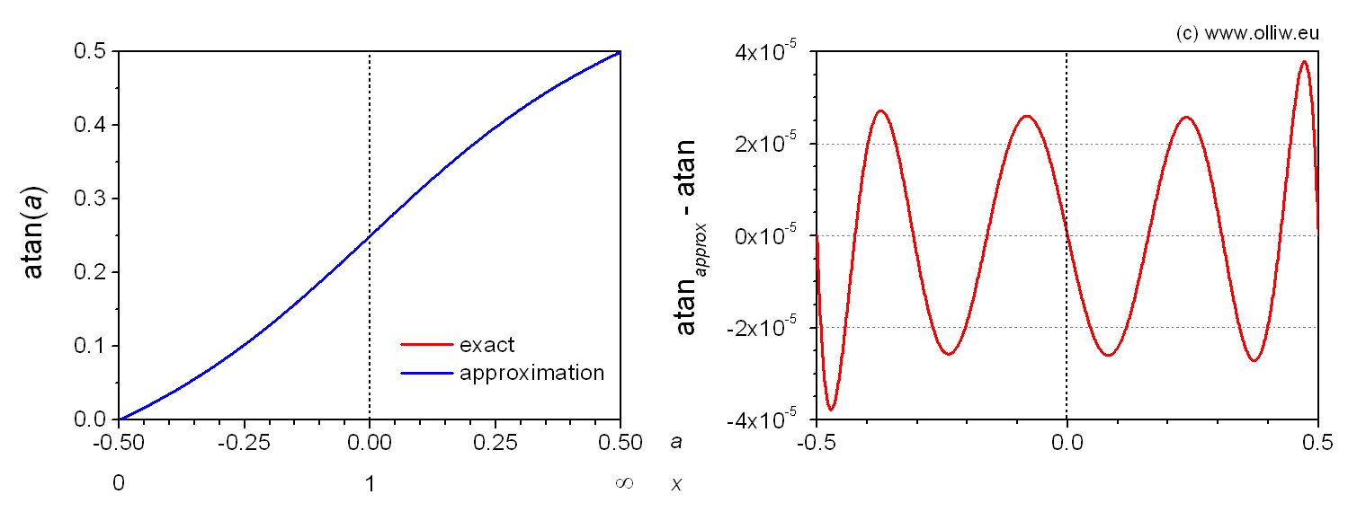
Funnily, the arctan is a very straight function for , and accordingly astonishingly simple and yet surprisingly accurate approximations are found on the web. The rational polynomial approximations I found most notable (e.g. here, here, here, here). However, it’s somewhat cumbersome to extend them to match my accuracy requirements, and they involve a division. So, I went with the „traditional“ approach of using a polynom.

|
I used a polynom of 7th order for sufficient accuracy. As for the sine and cosine, the „standard“ minimization schemes for finding the coefficients didn’t produced results I liked. I hence enforced the approximation to produce the correct values at the points  and used minimization for the remaining degrees of freedom. This resulted in
  
|
 
|
The absolute error is smaller than  (0.007°). Only 5 multiplications and 4 additions are required (not counting what’s needed to get ). The coefficients show alternating signs, and thanks to overflow doesn’t occur for the Q30 format.
Finally, a wrapper to calculate  may look as this (I followed the common definition, see here):
  if( x>0 ){

       if( y>=0 ){ //this ensures that |y+x| >= |y-x| and hence |a| <= 1

           a = q30_div( (y>>1) - (x>>1) , y + x );

           return q30_atan_normalized( a );

       }else{ //this ensures that |y-x| >= |y+x| and hence |a| <= 1

           a = q30_div( (y>>1) + (x>>1) , y - x );

           return -q30_atan_normalized( a );

       }

   }

   if( x<0 ){

       if( y>=0 ){

           a = q30_div( (y>>1) + (x>>1) , y - x );

           return Q30(1.0) - q30_atan_normalized( a );

       }else{

           a = q30_div( (y>>1) - (x>>1) , y + x );

           return q30_atan_normalized( a ) - Q30(1.0);

       }

   }

   if( y>0 ) return Q30(+1.0);

   if( y<0 ) return Q30(-1.0);

   return Q30(0.0);
3. Fast Arcsin
Finding a fast algorithm for the arcsin really presented a challenge, and caused some headaches. Any approximation is troubled by the  divergency at
  . In fact, all ideas I found on the web involve the calculation of a square-root at some point. For instance, one may first remove the square-root divergency from the original function, using formulas such as
 ,
,  ,
, 
and then approximate  (see e.g. here or here)(in particular the 3rd approach I found fascinating and to work very well). One may also use trigonometric relations such as
 ,
, 
and use a fast arctan method. Lastly, one may branch and use a polynomial approximation for, e.g.,  and obtain the values for
  from relations such as

Fast floating-point (inverse) sqrt algorithms are available, since thanks to the special structure of a floating-point very good seeds for Newton iterations can be obtained easily with „magic numbers“. However, for fixed-point values a sqrt calculation is at least as costly (if not many times more) as any polynomial approximation. In short, the sqrt necessarily makes the algorithm quite slow, at least as compared to the sin, cos, and arctan methods.
I didn’t liked that. I didn’t liked that at all, and hence decided to trade for a compromise. The underlying idea is that the arcsin is needed to calculate one of the Euler angles, namely exactly that one which also presents the gimbal lock issue. The bottom line is that one actually doesn’t need a good approximation near or angles of  , since either the calculation breaks down near those angles anyhow, or one would switch to another representation.
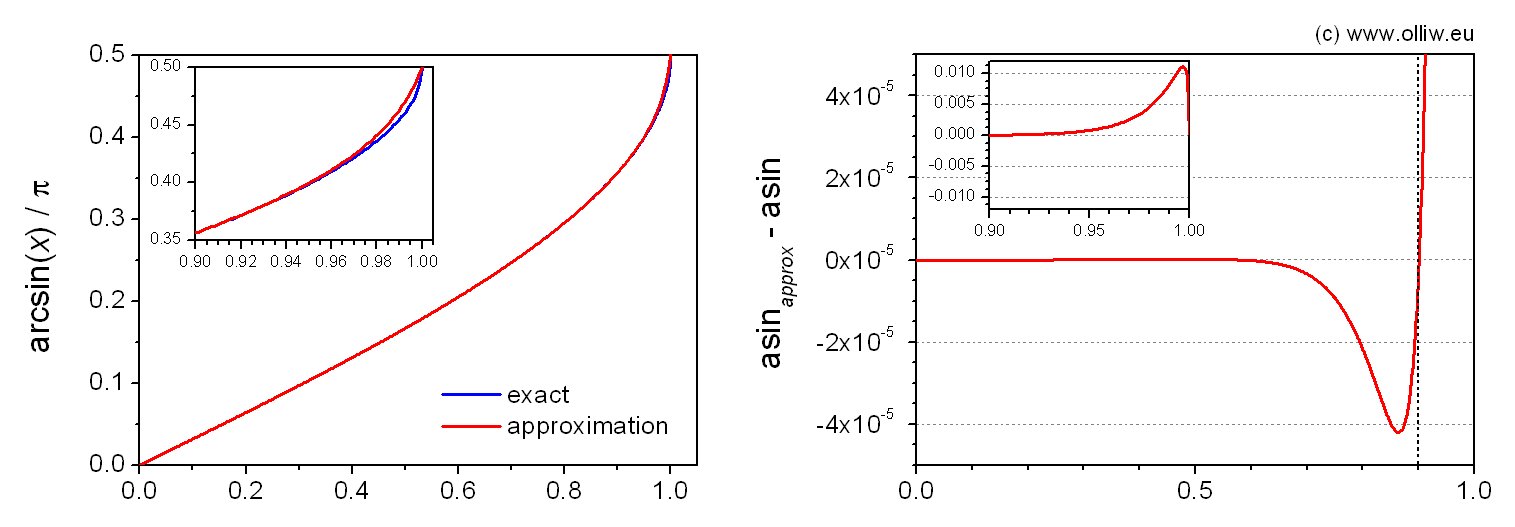
So, I went for a rational polynomial approximation and only ensured that it is well behaved (by e.g. forcing it to produce the correct values at ), but allowed for a poor absolute accuracy near . In addition I normalized the output values to , i.e. defined  .
.
That’s what I came up with after many trials:

|
Mathematically, either  or
or  is superfluous and can be set to one, but I kept them for numerical reasons. The coefficients I have determined such, that I enforced the approximation to reproduce the correct values for
  and
and  , as well as the correct Taylor expansion coefficients at up to 7th order. This left one degree of freedom, which I tuned by hand. The result is:
   
|
   
|
The absolute error is smaller than  up to
up to  , smaller than
  (0.008°) up to
  , and maximal
  at
at  , but the output never exceeds 1. One division and 9 multiplications are required. The coefficients show alternating signs and are small, and the calculation of the polynomials is stable without overflows. However, a slight issue is that the numerator and denominator polynomials both become quite small towards
  (of about 0.005), and a loss of precision may occur in the division. However, the Q30 format has by far sufficient resolution. Also, one could scale up both polynomials when their value falls below a threshold of e.g. 0.01. Anyway, in practice I found the above algorithm to work very well.
4. Fast Inverse Sqrt
Finding a suitable sqrt or inverse sqrt algorithm was easy, since I played it simple. In the AHRS calculations the sqrt is needed to normalize vectors, quaternions, and so on. In any working algorithm their magnitudes are close to one in any case, and just need to be renormalized. So, one just needs a method which works well for values close to one, which obviously simplifies the task. Two approaches come immediately to mind.
Firstly, one may use a Tayler series expansion of  around . The error of odd-order expansions is however such, that the magnitude of the normalized quantity can be larger than 1, which is quite unfavorable for AHRS calculations. This suggests to use the 2nd order approximation:

Secondly, one may use Newton iteration with the seed  . For the inverse square-root the iteration is in fact extremely simple, as it involves only addition and multiplication, and no division:

Nicely enough, its error is such that the magnitude of the normalized quantity is always smaller (or equal) to 1.
With two Newton steps, 3 multiplications are needed as compared to 2 for the 2nd-order Taylor series, but the accuracy is much better, and even better than that of the 3rd-order Taylor series. With three Newton steps, requiring 6 multiplications, the accuracy is already better than  in the range of
  . I settled for the Newton with 2 iterations.
  // y1 = 3/2 - 1/2*x

   y = Q30(1.5) - (x>>1);

   // y2 = (1.5 - x * y1* (y1/2) ) * y1

   y =  q30_mul( Q30(1.5) - q30_mul( x, q30_mul(y,y>>1) ) , y );

   return y;
The last line can be repeated for any further step if required.
6 Kommentare