OlliW's Bastelseiten » Brushless Gimbal Direct Drive: Theory and Experiment

I too got excited about the recent development of the brushless direct drive gimbals, pioneered by AlexMos. So far, all DIY or commercial solutions (I know about) are for cameras of the GoPro size or larger, but I was interested in building a gimbal for cameras of the key chain type, i.e. a micro brushless gimbal. I did encounter, however, various problems, and so I went into trying to understand better the brushless direct drive. My considerations and results please find below.

1. Basic experimental observations
2. Theory
2.1. Three-phase motor model, 2.2. Sinusoidal motor drive, 2.3. Direct-drive motor model, 2.4. Gimbal model
3. Typical cases and comparison to experiment
3.1. Static behavior, 3.2. Small angle behavior, 3.3. Behavior at constant speed
4. Model estimation and validation
5. Conclusions
Appendix A.1, A.2

1. Basic experimental observations

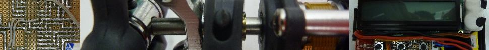
As a first step towards a micro gimbal I investigated several motors for their suitability, and I ended up with the PS2 Slim disc drive motor. It needs to be rewound and slightly remodeled (for details on the motor see here). Using this motor and a keychain camera I made a 1-axis gimbal for testing. Three observations I found key to better understand the brushless direct drive:

(1) Static angle deflection
If the motor is driven such as to hold a certain position, but a mechanical torque is applied to it, then the motor will turn somewhat to avoid the torque. If the torque is removed the motor will return to its original position. The stiffness, with which the motor reacts to a torque, is the stronger the larger the applied voltage. If, however, the torque becomes too large then the motor will snap into a new minimum position. It’s like scraping with a stick across a washboard, where the height of the ripples is given by the voltage and the period by the number of motor poles.

These observations are of course totally expected and easily understood; they characterize the static behavior. The motor stiffness determined by this experiment is an important motor parameter.

(2) Oscillatory step response
If the motor is driven such as to hold a certain position, and the gimbal is first deflected (by e.g. tapping it with a finger) but then released, then the motor will return to its original position within a certain time. For my gimbal setups, the motor returns with a pronounced oscillatory behavior. The gimbal (motor+mount+camera) is thus characterized as an under-damped second-order process.

The gimbal oscillation frequency and damping coefficient are important motor parameters, characterizing the dynamic behavior.

(3) Locking into oscillations at large drive speeds
If the motor is driven such as to rotate at a fixed speed, then the motor can get into a situation where it doesn’t move forward anymore but oscillates permanently around a certain position. For this to happen the speed has to be above a threshold speed. The oscillation frequency is the faster and the amplitude the smaller the larger the nominal drive speed is. This non-advancing oscillatory state can be reached by e.g. taping the camera to hold, or by trying to speed up the motor too fast.

These observations indicate that the gimbal system is highly non-linear. They came as a surprise to me, and it had in fact been these findings, and my desire to understand them, which triggered all the work presented here :-).

This video shows phenomenon (3):

I have also build a 1-axis test gimbal using a EMax CF2822 (12n14p, rewound 75 turns, 15 Ohms) and a Lumix (ca. 150g) camera, for which I made also observations (1) and (2) [I did not check for (3)].

2. Theory

The starting point for the theory of the brushless direct drive is the observation, that the brushless motor is essentially used as a 3-phase synchronous motor, and is driven by applying a 3-phase sinusoidal voltage to the phases. I won’t go into this here; I assume that this is well understood by the reader.

2.1. Three-phase motor model
The following motor model can be found in any introductory text on 3-phase motors:

$\left(\begin{array}{c} \Psi_a\\\Psi_b\\\Psi_c \end{array}\right) = L^w \left(\begin{array}{c} i_a\\i_b\\i_c \end{array}\right) + L^v \left(\begin{array}{ccc} 0&-1&-1\\-1&0&-1\\-1&-1&0 \end{array}\right) \left(\begin{array}{c} i_a\\i_b\\i_c \end{array}\right) + \left(\begin{array}{c} \Psi_{pa}\\\Psi_{pb}\\\Psi_{pc} \end{array}\right)$ Eq. (2.1)

$\left(\begin{array}{c} U_a\\U_b\\U_c \end{array}\right) = R^w \left(\begin{array}{c} i_a\\i_b\\i_c \end{array}\right) + \dfrac{d}{dt} \left(\begin{array}{c} \Psi_a\\\Psi_b\\\Psi_c \end{array}\right)$ Eq. (2.2)

$\left(\begin{array}{c} \Psi_{pa}\\\Psi_{pb}\\\Psi_{pc} \end{array}\right) = \Psi_p \left(\begin{array}{c} \cos\epsilon\\\cos(\epsilon-\frac{2\pi}{3})\\\cos(\epsilon-\frac{4\pi}{3}) \end{array}\right)$ Eq. (2.3)

The angle $\epsilon$ denotes the electrical angle of the motor’s rotor. It is related to the mechanical angle $\epsilon_m$ via the number of motor pole pairs $p$ : $\epsilon_m = \epsilon/p$ . With the transformation $abc \to \alpha\beta$ the equations read:

$\left(\begin{array}{c} \Psi_\alpha\\\Psi_\beta \end{array}\right) = L \left(\begin{array}{c} i_\alpha\\i_\beta \end{array}\right) + \Psi_p \left(\begin{array}{c} \cos\epsilon\\\sin\epsilon \end{array}\right)$ with $L=L^w + L^v$ Eq. (2.4)

$\left(\begin{array}{c} U_\alpha\\U_\beta \end{array}\right) = R \left(\begin{array}{c} i_\alpha\\i_\beta \end{array}\right) + \dfrac{d}{dt} \left(\begin{array}{c} \Psi_\alpha\\\Psi_\beta \end{array}\right)$ with $R=R^w$ Eq. (2.5)

$M = \dfrac{3}{2} \Psi_p \left( i_\beta \cos\epsilon - i_\alpha\sin\epsilon \right)$ Eq. (2.6)

And with the transformation $\alpha\beta \to dq$ one obtains:

$\left(\begin{array}{c} \Psi_d\\\Psi_q \end{array}\right) = L \left(\begin{array}{c} i_d\\i_q \end{array}\right) + \Psi_p \left(\begin{array}{c} 1\\0 \end{array}\right)$ Eq. (2.7)

$\left(\begin{array}{c} U_d\\U_q \end{array}\right) = R \left(\begin{array}{c} i_d\\i_q \end{array}\right) + \dfrac{d}{dt} \left(\begin{array}{c} \Psi_d\\\Psi_q \end{array}\right) + \dot{\epsilon} \left(\begin{array}{cc} 0&-1\\1&0 \end{array}\right) \left(\begin{array}{c} \Psi_d\\\Psi_q \end{array}\right)$ Eq. (2.8)

$M = \dfrac{3}{2} \Psi_p i_q$ Eq. (2.9)

Instead of the $dq$ representation I found it more convenient to express the $\alpha\beta$ equations using a complex notation, $\hat{x} = x_\alpha + j x_\beta = x_0 e^{j\varphi}$ (I haven’t seen this done in the literature I found on the web, but it’s probably quite standard). It results in

$\hat{\Psi} = L \hat{i} + \Psi_p e^{j\epsilon}$ Eq. (2.10)

$\hat{U} = R \hat{i} + \dfrac{d}{dt} \hat{\Psi} = R \hat{i} + L \dfrac{d}{dt} \hat{i} + j \Psi_p \dot{\epsilon} e^{j\epsilon}$ Eq. (2.11)

$M = \dfrac{3}{2} \Psi_p \text{Im}[ \hat{i} e^{-j\epsilon}]$ Eq. (2.12)

2.2. Sinusoidal motor drive
Next we have to describe the sinusoidal motor drive, which is simple enough. The motor drive applies three voltages to the motor, with amplitudes $(U_a,U_b,U_c) = U_0 [\cos\theta,\cos(\theta-\frac{2\pi}{3}),\cos(\theta-\frac{4\pi}{3})]$ . The angle $\theta$ determines the position at which the motor is supposed to be, and it is our control variable for moving the motor. The applied voltages lead to currents, which may however not be in phase with the voltages, and hence are characterized by another angle $\zeta$ . In complex notation we obtain:

$\hat{U} = U_0 e^{j\theta}$ $\hat{i} = i_0 e^{j\zeta}$ Eq. (2.13)

2.3. Direct-drive motor model
Using Eq. (2.13) our motor is thus described by

$U_0 e^{j(\theta-\epsilon)} = ( R + j L \dot{\zeta} ) i_0 e^{j(\zeta-\epsilon)} + j k \dot{\epsilon}$ Eq. (2.14)

$M = \dfrac{3}{2} k \text{Im}\left[ \dfrac{ U_0 e^{j(\theta-\epsilon)} - j k \dot{\epsilon}}{R + j L \dot{\zeta}}\right]$ Eq. (2.15)

where I have set $k= \Psi_p$ in order to be more consistent with usual notation of motor parameters. For our purposes we may simplify Eqs. (2.14) and (2.15), since the motor will never be driven at high rotation speeds, and hence $\omega \ll R/L$ . We arrive at the direct-drive motor model:

$M = \dfrac{3}{2} \dfrac{k}{R} \left[ U_0 \sin(\theta-\epsilon) - k \dot{\epsilon} \right]$ Eq. (2.16)

2.4. Gimbal model
Finally we have to take into account the mechanical properties of the motor and the camera attached to it. The mechanical dynamics of both can be described by a moment of inertia $T$ , and some friction:

$T \ddot{\epsilon} = M_{motor} - a |\epsilon| - b \dot{\epsilon}$ Eq. (2.17)

Please note that I have used here the electrical rotation angle, and not the mechanical angle. I will assume $a=0$ in the following. We thus arrive at the equation of motion:

$T \ddot{\epsilon} + \left(\dfrac{3k}{2R}k+b \right) \dot{\epsilon} - \left(\dfrac{3k}{2R} U_0 \right) \sin(\theta-\epsilon) = 0$ Eq. (2.18)

which is that of a driven damped non-linear oscillator ( $\theta$ is the drive). The sine-type non-linearity is well known from the physical pendulum, and we will strongly profit from the results available for it. We thus write also

$\ddot{\epsilon} + 2 \gamma \dot{\epsilon} + \omega_0^2 \sin(\epsilon-\theta) = 0$ Eq. (2.19)

$\omega_0^2 = \dfrac{3k}{2R} \dfrac{U_0}{T}$ $\gamma = \dfrac{ \frac{3k}{2R} k + b }{2T}$ $Q = \dfrac{1}{2d} = \dfrac{\omega_0}{2\gamma} = \dfrac{ \sqrt{U_0 T} }{ \sqrt{\frac{3k}{2R}} k + \sqrt{\frac{2R}{3k}} b }$ Eq. (2.20)

3. Typical cases and comparison to experiment

Having established the model for the direct-drive gimbal, Eqs. (2.18) and (2.19), we can discuss some typical situations. In fact, we can consider now exactly those three cases presented in Chapter 1.

3.1. Static behavior
The direct-drive motor model Eq. (2.16) neatly explains observations (1). When a not too large torque is applied to the motor, a difference occurs between position $\theta$ as commanded by the motor drive and actual position $\epsilon$ of the motor. Moreover, the lag is the more pronounced the larger the torque. The stiffness at small torques is given by

$\epsilon = \theta - \left( \dfrac{3k}{2R} \right)^{-1} \dfrac{M}{U_0}$ Eq. (3.1)

which emphasized the relevance of the parameter $\frac{3k}{2R}$ . If the torque is too large, the motor will slip, since the sine function is bounded.

3.2. Small angle behavior
If the difference between commanded angle $\theta$ and motor position $\epsilon$ is small we may approximate the sine in Eqs. (2.18) or (2.19), which leads to the damped driven harmonic oscillator:

$\ddot{\epsilon} + 2 \gamma \dot{\epsilon} + \omega_0^2 \epsilon = \omega_0^2 \theta$ Eq. (3.2)

Notably, the strength of the drive is not an independent variable, but is given by the oscillation frequency itself. From this equation we may derive the transfer function

$H(s) = \dfrac{\omega_0^2}{ s^2 + 2d \omega_0 s + \omega_0^2 }$ Eq. (3.3a)

$F(\omega) = \dfrac{ 1}{ 1 + j 2 d \dfrac{\omega}{\omega_0} - \left(\dfrac{\omega}{\omega_0}\right)^2 }$ Eq. (3.3b)

showing that the gimbal represents a second order process. It may be over-damped then $d>1$ (which is good for control) or under-damped then $d<1$ (which is harder for control).

As expected, the resonance frequency increases (i.e. the system becomes faster) with increasing voltage amplitude $U_0$ (stronger motor) as well as with decreasing moment of inertia $T$ (gimbal/camera easier to turn). Interestingly, since somewhat unexpected, the system becomes less damped with higher voltages, which may explain why for a given setup smaller voltages yield a better gimbal performance (as control is easier).

For my micro and Lumix test gimbals I observe strongly under-damped oscillations in a step response experiment [observation (2) in Chapter 1], i.e., the parameters are unfortunately such that $d$ is quite small.

3.3. Behavior at constant speed
This case is, from an intellectual point of view, most interesting. I found it convenient to switch to the new variable $\delta = \theta - \epsilon$ , which can be regarded as the phase lag. Then Eq. (2.19) becomes

$\ddot{\delta} + 2 \gamma \dot{\delta} + \omega_0^2 \sin(\delta) = \ddot{\theta} + 2 \gamma \dot{\theta}$ Eq. (3.4)

Driving the motor at constant speed corresponds to $\theta(t) = \Omega t$ , implying $\ddot{\theta}=0$ and $\dot{\theta} = \Omega$ . With damping neglected, which is sufficient for grasping the general behavior, we arrive at

$\ddot{\delta} + \omega_0^2 \sin(\delta) = 0$ Eq. (3.5)

Hence, the phase lag $\delta$ behaves like a non-linear oscillator, with a standard sine-type non-linearity. We immediately infer two different solutions:

(1) For small phase lags or $\sin(\delta) \approx \delta$ , $\delta$ oscillates harmonically with frequency $\omega_0$ : $\delta(t) \propto \cos( \omega_0 t)$ (see e.g. this animation). That is, the motor advances with speed $\Omega$ , but with harmonic oscillations superimposed: $\epsilon(t) = \Omega t + A \cos( \omega_0 t + \varphi_0)$ . The amplitude $A$ , or energy $E$ of the pendulum, is small for small speeds, but increases with speed. In the video shown in Chapter I the superimposed oscillations are observed as a sort of stuttering at intermediate speeds (below the threshold speed).

(2) The pendulum may be excited strongly, such that it permanently overturns (see e.g. this animation). The phase lag hence advances constantly with a non-harmonic periodic function superimposed: $\delta(t) = \Omega t + f(\omega t)$ , where $\omega$ is non-trivially obtained. Hence, the motor is not advancing but oscillates around a fixed position: $\epsilon(t) = f(\omega t)$ . The amplitude of the oscillation $f$ decreases with larger energy of the pendulum or speed $\Omega$ .

The crossover between the two regimes occurs at the point there the pendulum has just enough energy to complete a full swing (see e.g. this animation) (in the phase space diagram this is the separatix), and which situation occurs is controlled by the energy $E$ of the pendulum. The energy in turn is roughly determined by the square of the speed, $E \propto \Omega^2$ .

These findings explain nicely all observations (3) in Chapter 1.

4. Model estimation and validation

Using the micro gimbal test setup I recorded the step response for four different voltages. More precisely, the motor was driven using the L6234 driver IC at 3S, and the H bridges of the L6234 were driven with PWM signals with 8 bit resolution at 8 kHz. The different voltages were set via different maximal PWM duty cycles. Vmax = 100 e.g. corresponds to a duty cycle of 100/256. A step of amplitude „100“ was applied, which corresponds to a 100/252 * 60° = 23.8° mechanical turn of the gimbal. The angle was determined by integrating the gyro signal (MPU6050) taken every 1 ms, the angle value was however recorded „only“ every 5 ms. The gyro setting was DLPF 256, FS 1000, SR 0. I repeated the measurements several times and found good reproducibility. The curves for the four voltages Vmax = 200, 100, 50, and 25 are shown in the following diagram. The step occured at time t = 0.

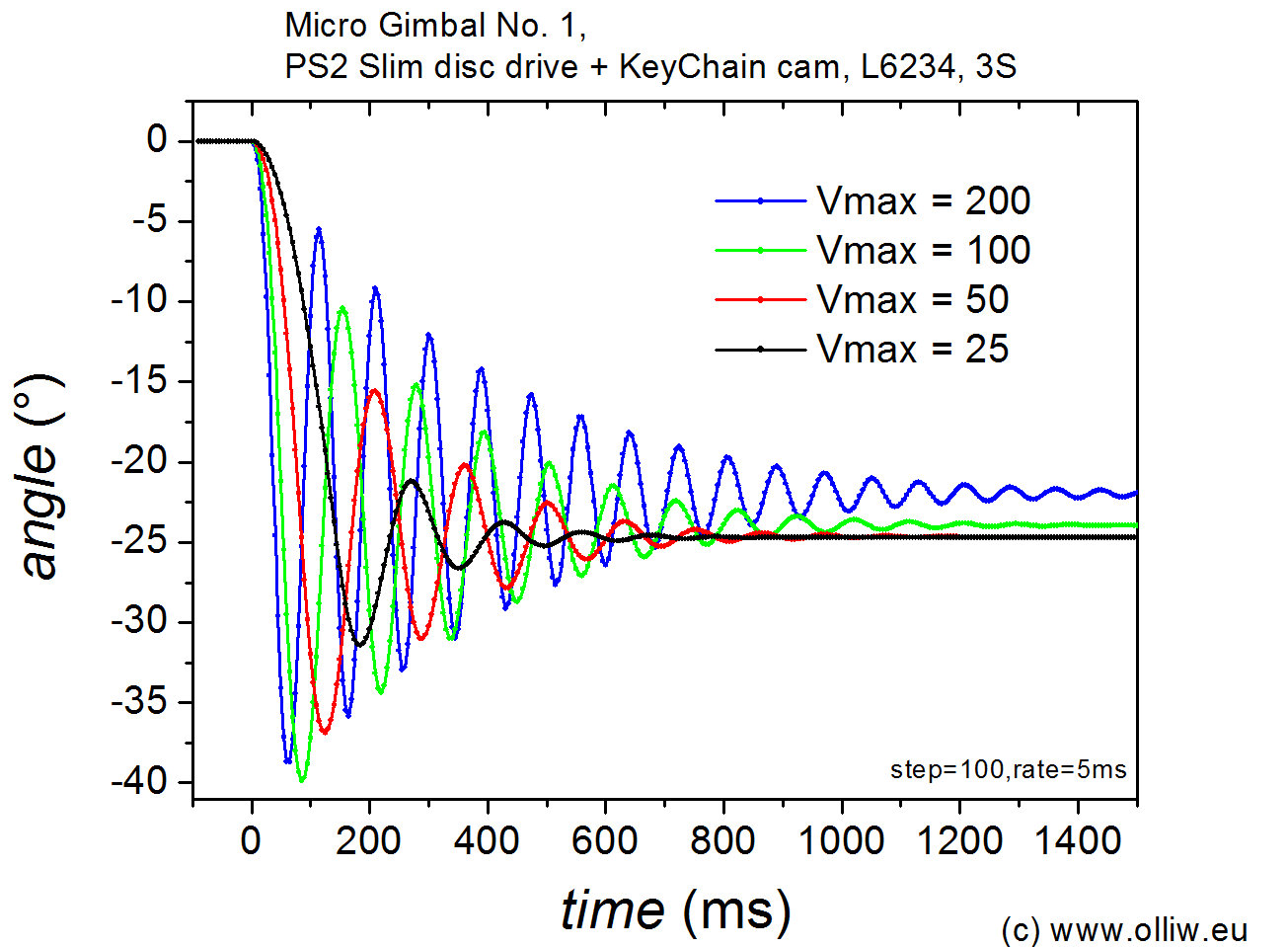
The oscillatory response corresponding to a highly under-damped second-order process is clearly observed. Furthermore, the above trends are clearly seen: The higher the voltage the larger the frequency and the smaller the damping. Taking into account that the derived model is also able to reproduce observations (1) and in particular observations (3) described in Chapter 1, we can conclude that the model captures the behavior of the real gimbal quite well, at least on a semi-quantitative level.

Quantitatively, some discrepancies are observed. The damped oscillations are reasonably but not perfectly fitted by a damped harmonic oscillator; the period shifts somewhat during the relaxation, and the damping is not perfectly exponential. This can be, however, due to many reasons, e.g. the friction model is too simplistic, the non-linearity is not of sine-type e.g. due to cogging torque moments, or the process is higher-order. Also, a step of „100“ or 23.8° might be too large for the considered linear regime to hold (I might repeat the measurements for smaller steps, but I find the above results convincing enough). To give some numbers, the resonance frequency $f_{res}$ decreases from ca. 12 Hz at Vmax = 200 to ca. 7 Hz at Vmax = 25, and the damping $d$ increases from ca. 0.04 to ca. 0.15.

The step responses do not settle at 23.8° for the larger voltages. I was suspecting that this comes from the limited gyro bandwidth, which introduces integration errors. I am not sure about it, however.

For the test gimbal with the Emax CF2822 and Lumix camera I obtained very similar data, only that the frequencies are generally somewhat smaller, it is ca. 7 Hz at Vmax = 200. The same trends are however observed.

5. Conclusions

The above results demonstrate the challenges in controlling direct-drive gimbals using PID controllers. The process is rarely strongly over-damped, where the transfer function could be approximated by a model with a dominating time constant. In contrast, the process is nearly critical or even strongly under-damped as in the case of my micro and Lumix test gimbals, and tuning is much „harder“ since a complex or nearly complex pair of poles needs to be compensated for instead of only one real pole. This implies that the conventional rules for tuning PID controllers do not apply, and that the feedback loop is quite sensitive to parameter variations. Using a parameterization of the P, I, D values which is better adapted to oscillatory second-order plants might simplify the tuning process.

Appendix

A.1. DC motor direct drive
It is interesting for comparison to look also briefly at the situation of a direct drive using an ordinary (brushed) DC motor. The DC motor equations are

$U = R I + L \dot{I} + k \omega$ Eq. (A1.1)
$M = k I$ Eq. (A1.2)

and the mechanical properties are described as before by Eq. (2.17), i.e.

$T \dot{\omega} = M_{Motor} - b \omega$ Eq. (A1.3)

where again $a=0$ was set. One thus arrives at the equation of motion

$\ddot{\omega} + \left(\dfrac{RT+Lb}{LT} \right) \dot{\omega} + \left(\dfrac{Rb+k^2}{LT} \right) \omega = \left(\dfrac{k}{LT}\right) U$ Eq. (A1.4)

This is again a second-order differential equation, corresponding to second-order transfer functions, as for the brushless drive. However, despite the seeming similarity, the two cases are quite different. First, the equation of motion and/or transfer function for the DC drive refers to angular speed $\omega$ , while those for the brushless drive refer to angular position $\epsilon$ . Second, it is intrinsically linear. Finally, the second-order nature of Eq. (A.4) comes from taking into account the effects of inductance $L$ , which is usually negligible because of $\omega \ll R/L$ and/or using PWM. Accordingly, for the same reasons as in chapter 2.3, the appropriate equation of motion for describing a DC motor driven gimbal is in fact

$\dot{\omega} + \left(\dfrac{Rb+k^2}{RT} \right) \omega = \left(\dfrac{k}{RT}\right) U$ Eq. (A1.5)

and the transfer function with respect to the angular position $\epsilon$ reads

$\epsilon(s) = \dfrac{K}{s(1+\tau s)} U(s)$ Eq. (A1.6)

This is a second-order process as for the brushless direct-drive gimbal, but with the crucial difference that the resonance frequency $\omega_0$ is zero. That is, the DC motor direct-drive method is intrinsically over-damped.

A.2. Torque controlled direct drive
The discussion of the DC motor direct drive in chapter A.1 suggests another interesting situation of a direct drive. Usually, a DC motor is controlled via the applied voltage, as in chapter A.1. However, it may also be driven by controlling the current $I$ . As Eq. (A1.2) shows, this essentially corresponds to controlling the torque, which is applied to the gimbal. This case is also described by Eqs. (A1.1), (A1.2), and (A1.3), but now the transfer function as function of current $I$ (and not of voltage $U$ ) is of relevance. Assuming again $a=0$ one directly obtains the equation of motion

$\dot{\omega} + \left(\dfrac{b}{T} \right) \omega = \left(\dfrac{k}{T}\right) I$ Eq. (A2.1)

and the transfer function

$\epsilon(s) = \dfrac{K}{s(1+\tau s)} I(s)$ . Eq. (A2.2)

Note, in contrast to the voltage-controlled DC motor direct drive a low-frequency assumption was not necessary; the results hold here for all frequencies. Besides that, one obtains also an over-damped second-order process with zero resonance frequency $\omega_0$ . Hence, controlling the current or torque, respectively, should be an attractive approach for direct drive gimbals.

B. Formulary

Clark Transformation, $abc \to \alpha\beta$ , and Inverse

$\left(\begin{array}{c} \alpha \\ \beta \end{array}\right) = \dfrac{2}{3} \left(\begin{array}{ccc} 1 & -\frac{1}{2} & -\frac{1}{2} \\ 0 & \frac{\sqrt{3}}{2} & -\frac{\sqrt{3}}{2} \end{array}\right) \left(\begin{array}{c} a\\b\\c \end{array}\right)$ Eq. (B.1)

$\left(\begin{array}{c} a\\b\\c \end{array}\right) = \left(\begin{array}{cc} 1 & 0 \\ -\frac{1}{2} & \frac{\sqrt{3}}{2} \\ -\frac{1}{2} & -\frac{\sqrt{3}}{2} \end{array}\right) \left(\begin{array}{c} \alpha \\ \beta \end{array}\right)$ Eq. (B.2)

Note:

$\bf{C} \left(\begin{array}{ccc} 0 & -1 & -1 \\ -1 & 0 & -1 \\ -1 & -1 & 0 \end{array}\right) = \bf{C}$

Park Transformation, $\alpha\beta \to dq$

$\left(\begin{array}{c} d\\q \end{array}\right) = \left(\begin{array}{cc} \cos \epsilon & \sin \epsilon \\ -\sin \epsilon & \cos \epsilon \end{array}\right) \left(\begin{array}{c} \alpha \\ \beta \end{array}\right)$ Eq. (B.3)

Note:

$\bf{P} \left(\begin{array}{c} \cos\epsilon \\ \sin\epsilon \end{array}\right) = \left(\begin{array}{c} 1 \\ 0 \end{array}\right)$

$\bar{U} = \hat{U} e^{-j\epsilon}$

Combined Clark-Park Transformation, $abc \to dq$ , and Inverse

$\left(\begin{array}{c} d \\ q \end{array}\right) = \dfrac{2}{3} \left(\begin{array}{ccc} \cos\epsilon & \cos(\epsilon-\frac{2\pi}{3}) & \cos(\epsilon-\frac{4\pi}{3}) \\ -\sin\epsilon & -\sin(\epsilon-\frac{2\pi}{3}) & -\sin(\epsilon-\frac{4\pi}{3}) \end{array}\right) \left(\begin{array}{c} a\\b\\c \end{array}\right)$ Eq. (B.4)

$\left(\begin{array}{c} a\\b\\c \end{array}\right) = \dfrac{2}{3} \left(\begin{array}{cc} \cos\epsilon & -\sin\epsilon \\ \cos(\epsilon-\frac{2\pi}{3}) & -\sin(\epsilon-\frac{2\pi}{3}) \\ \cos(\epsilon-\frac{4\pi}{3}) & -\sin(\epsilon-\frac{4\pi}{3}) \end{array}\right) \left(\begin{array}{c} d \\ q \end{array}\right)$ Eq. (B.5)

Transformation Examples

$\left(\begin{array}{c} a \\ b \\ c \end{array}\right) = U \left(\begin{array}{c} \cos\theta \\ \cos(\theta-\frac{2\pi}{3}) \\ \cos(\theta-\frac{4\pi}{3}) \end{array}\right)$

$\rightarrow \left(\begin{array}{c} \alpha \\ \beta \end{array}\right) = U \left(\begin{array}{c} \cos\theta \\ \sin\theta \end{array}\right)$ , $\hat{U} = U e^{j\theta}$

$\rightarrow \left(\begin{array}{c} d \\ q \end{array}\right) = U \left(\begin{array}{c} \cos(\theta-\epsilon) \\ \sin(\theta-\epsilon) \end{array}\right)$ , $\bar{U} = U e^{j(\theta-\epsilon)}$

$\hat{U} = R \hat{i} + L \dfrac{d}{dt} \hat{i} + j \Psi_p \dot{\epsilon} e^{j\epsilon}$ , $M = \dfrac{3}{2} \Psi_p \text{Im}[ \hat{i} e^{-j\epsilon}]$

$\bar{U} = R \bar{i} + L \dfrac{d}{dt} \bar{i} + j \dot{\epsilon} (L \bar{i} + \Psi_p )$ , $M = \dfrac{3}{2} \Psi_p \text{Im}[ \bar{i} ]$

Brushless Gimbal Direct Drive: Theory and Experiment

2 Kommentare

Hinterlasse einen Kommentar Antworten abbrechen

Artikel Auswahl

Suche

Login

Impressum

Blogroll

Themen

Seiten