1. Theory
1.1. Propeller
The static thrust  generated by the propeller and the mechanical power
  required to spin the propeller are given by
 ,
,
 ,
,
where  is the density of air,
  is the diameter of the propeller, and
  is the angular velocity of the rotation. The power is related to the mechanical torque
  for spinning the propeller as
 .
.
The thrust and mechanical power are thus related as
 ,
,
where  can be identified as the efficiency of the propeller, defined as
  , and is obtained as
 .
.
Comments: It should be noted that the coefficients  and
and  introduced here differ by constant factors from definitions found in the literature. It also should be mentioned that in general these coefficients, and whereby the propeller efficiency, can be dependent on the rotation speed .
1.2. Motor
The mechanical power is delivered by the motor, which is reasonably well described by the classical motor equations, which in the static case read
 ,
,
 ,
,
where  and
and  are the motor constants (related to the KV value),
  is the resistance of the wires, and
  accounts for additional losses such as friction or iron core losses, and is typically rotation speed dependent. Common approximations are
  , or
, or  , or in the simplest case just
  (the so called „half-ideal“ motor). Often also
  is assumed (or a similar fixed relation in case of multi-phase motors).
1.3. Model
With , one immediately arrives at
 .
.
With introducing a coefficient  as
as
 ,
,
one thus arrives at the main result of this article:
 .
.
This equation implies that the thrust generated by the propeller can be estimated from measurements of the rotation speed and the current through the motor. For the purpose of compensating the thrust characteristic the absolute value of the coefficient is irrelevant, as only normalized quantities would be used. For the same reason, the conversion factor from to  is irrelevant. One thus arrives at the practical relation
 ,
,
where  is a normalized thrust and the dependence on
  has been made explicit.
1.4. Model Assumptions
The derived relationship involves two approximations, namely the assumption of and that the propeller efficiency is constant and not dependent on the rotation speed, which both need to be justified or validated.
Comment: Note that the efficiency of the motor does not enter in these equations and is thus irrelevant.
In case of it can be argued that for a good motor these losses should be small, i.e., that the largest loss contribution is the Joule’s heating due to the motor resistance . If this is found to not be true for a particular motor, then this could be easily accounted for in the treatment by extending the above equation accordingly; one could e.g. subtract a current  from the measured current.
In case of it can be argued that it’s value generally doesn’t vary much. For instance, in [SCH] the efficiency of a bad propeller was assigned to ca.  , and to ca.
  for a good propeller. In [DET] the efficiency of very small propellers ranged in ca. 0.4 – 0.6. Expecting an essentially constant propeller efficiency thus doesn’t look unreasonable a-priori. Indeed, in [DET], [BREa], [BREb] the coefficients and were found to be nearly independent on rotation speed, implying constant propeller efficiency. However, they are not totally constant. To conclude, this point is certainly a crucial factor potentially limiting the accuracy of the proposed method, and thus warrants further analysis.
2. Application
According to the above relation, one needs to measure the rotation speed and the current through the motor, as function of the input signal to the ESC. Traditionally this would require building a dedicated measurement stand, and many such builds are described in the web, from simple to sophisticated.
However, thanks to the more recent development that ESCs themselves offer telemetry data, this task is enormously simplified, and readily available to everyone. One only needs to fix the copter to the ground, which for not too big copters is easily achieved by hands-on approaches, and spin up a motor with the propeller attached. In fact, the emerging availability of ESCs with telemetry, and that they typically report rotation speed and current, has inspired this whole work described in this article.
In my case I used a UC4H ESC node driving a KISS 32A ESC; for details on this setup please see Uavcan for Hobbyists: UC4H ESC-Actuator Node. The KISS 32A ESC does provide telemetry, which is polled by the UC4H ESC node in regular time intervals (e.g. 200 ms), and send out to the CAN bus, which is used to control the ESC node.
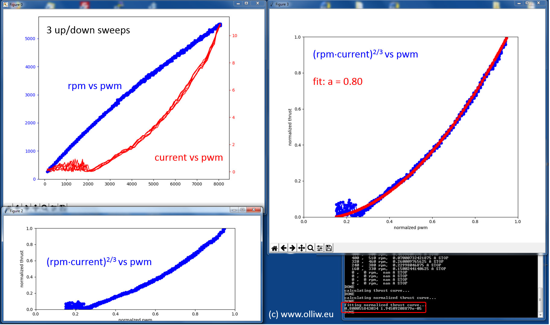
A Python script, making use of the PyUavcan library, controls the whole procedure (the script is available here): It ramps up and down the motor, e.g. three times, collects the telemetry data and plots them out, and finally uses the data to apply a fit to determine the MOT_THST_EXPO value, which is ArduPilot’s parameter for the internal thrust compensation.
The setup, and the result looked like this:

3. Model Validation
References
[BREa] Measurement of Static and Dynamic Performance Characteristics of Electric Propulsion Systems, by A. J. Brezina, 2012 [.pdf]
[BREb] Measurement of Static and Dynamic Performance Characteristics of Small Electric Propulsion Systems, by A. J. Brezina, S. K. Thomas, 2013 [.pdf]
[DET] Static Testing of Micro Propellers, by R. W. Deters, M. S. Selig, 2008 [.pdf]
[SCH] Der Standschub von Propellern und Rotoren, by H. Schenk, 2002 [.pdf]